|
Finally, I looked at my data through the lens of discriminant analysis. I was primarily interested to see if discriminant analysis could predict which of five, largely subjective breakage patterns a killed snail's shell would exhibit, based solely on my numerical variables. This would be interesting, because—if true—it would suggest that these patterns represent different hunting strategies that work optimally for crabs (or against snails) of particular sizes. The five categories of breakage I identified during the experiment were:
I adapted a series of R scripts from the website associated with the teaching text "The Little Book of R". Early on, I ran into problems. The script depends on a R package called MASS, which—after much trial and error—I discovered was incompatible with the package I was using to run my cluster analysis, vegan. MASS and vegan simply would not run in the same session of R. My solution, was to run my two different analyses in two different sessions of R, which seemed to work quite well. While not all aspects of the script could be adapted (notably, any attempt to group standardize the lda values leads to errors related to a number of unresolvable NAs), I was eventually able to produce several plots. The first of these, related to breakage pattern, is reproduced below. 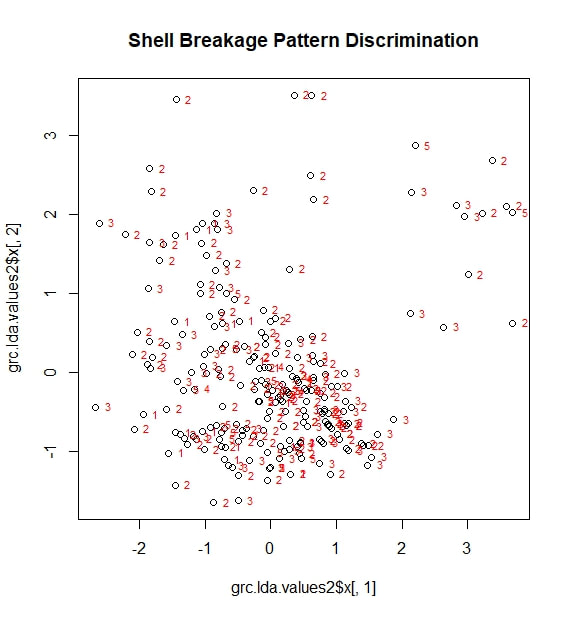 To my disappointment, no clear categories emerge. Looking at the scaling values for LD1, I found that it is primarily controlled (perhaps unsurprisingly) by largest surviving fragment ratio. This ratio also contributes strongly to LD2, along with shell thickness. In other words, the best tool for categorizing types of shell damage is, logically, a numerical measure of shell damage. However, even this straightforward tool is not enough to accurately predict the feeding strategy used during a particular predation event. Moving forward, I decided to see if any of my other categorical variables could be successfully parsed by discriminant analysis. I started with a long shot, trying to predict which individual predator (each with a numerical designation from 1 to 22) was involved in a feeding event. 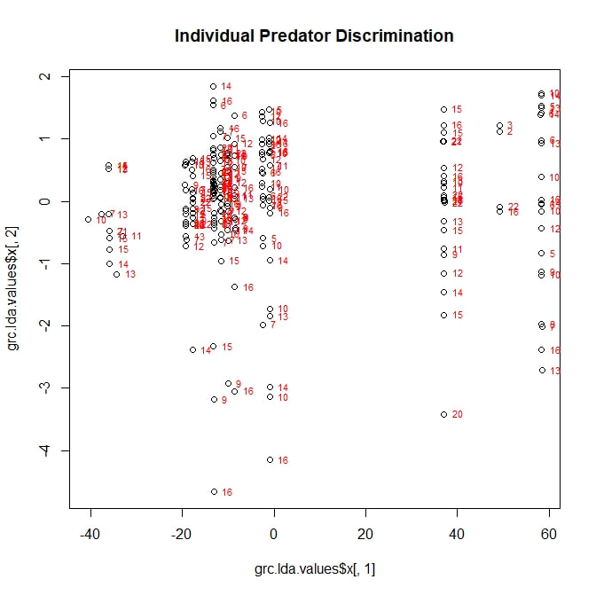 Initially, this analysis looked a little better. At least there were some distinctive groupings along LD1. However, once I superimposed the identification numbers of my individual predators, it became clear that these groupings did not represent any real ability to sort the data by predator. In passing, I will note that LD1 is largely based on carapace width (this makes sense; it is the one variable directly related to the predator, rather than the prey), while LD2 is related to largest fragment ration and to shell thickness. Next, I attempted what I assumed would be a more modest goal. Could discriminant analysis predict, based on my five variables, which attacks had been fatal? 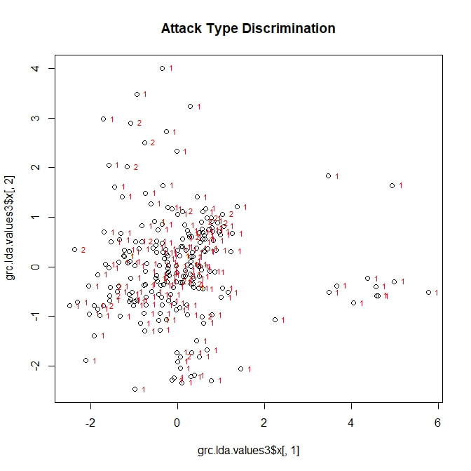 The answer: no. On the above figure, a point marked with a "1" represents a fatal attack, while a "2" represents a non-fatal, injurious attack (a third category "0", meaning "not attacked", is not here represented). LD1 is once more based on largest fragment ratio (logically, snails with more intact shells are more likely to be survivors of an attack) with minor contributions from shell thickness. LD2 is also based largely on largest fragment ratio. Neither factor adequately sorts the data into meaningful categories.
Finally, while it was impossible to plot the results of discriminant analysis based on prey species (with only two species, only one LDA scaling could be generated), I found that shell thickness was the best statistical tool for distinguishing one snail species from the other. All in all, this appears to be a data set resistant to discriminant analysis. Moving forward, I may try breaking my data out by prey species, as I have done elsewhere, or introducing new categorical variables to my data set such as predator size classes.
0 Comments
My next approach was to try cluster analysis, looking for meaningful groupings within my data set. I kept my five variables the same and again began without separating out my data by prey species. I adapted an R script (based on the package "vegan") to run several types of cluster analysis, including hierarchical and k-means, generating two dendrograms and an elliptical plot. Plotted together in one window, the result looks something like this: 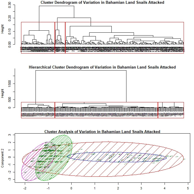 Each leaf or termination of the dendrogram represents a particular attack by a crab on a snail during this experiment. The boxes and ellipses represent the script's attempt to organize these feeding events to larger, meaningful categories. I have, somewhat arbitrarily, programmed the analysis to choose three such categories for each dendrogram and four for the elliptical plot. In both dendrograms we see one strongly differentiated group on the far left, and two more similar groups on the right. However, it is the bottom figure that I'd like focus on for the moment. The large red ellipse, I believe to be something of "wastebasket category", including as it does points from the extreme left and right of the spread. However, if I limit the analysis to three categories, the results are even more difficult to resolve. Largely ignoring, therefore, the red ellipse for the moment, let us consider the remaining groups. We have one strongly differentiated group (the blue) and two more similar groups (the green and the magenta), not so unlike what we see in the dendrograms. My suspicion, as yet unconfirmed, is that this repeated three-part signal is yet another prey species signal, with the single strongly differentiated grouping representing those Cerion snails killed during this experiment (as this group is smaller and the Cerion less numerous) and the other two groupings representing the H. varians. The two part H. varians signal is at least partly an artifact of my methods, but may also represent an ontogenetic signal. Snails ranged widely in size (and therefore presumptive maturity level) within H. varians, from as large as a nickel to smaller than one's littlest fingernail. I experimented to see if I could get a stronger prey species signal by limiting my analysis to prey body size variables, but the results were inconclusive. I therefore moved on to considering exclusively those attacks made against Cerion snails. 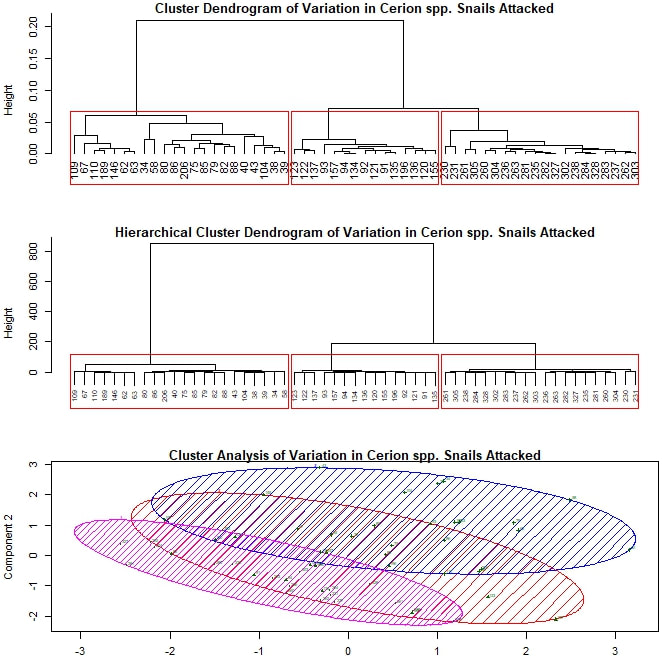 Here, as I continue with my somewhat arbitrary choice to divide the data set into three parts, patterns are harder to discern. All three elliptical groupings overlap quite closely, suggesting to me that these groups—unlike those seen previously—may not represent anything truly meaningful about the underlying data. Finally, I also performed a cluster analysis limited to the H. varians snails attacked during the experiment. 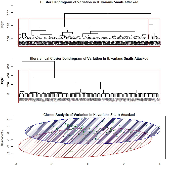 Here I was deliberately looking for two major groupings, hoping to replicate the (possibly ontogenetic) signal observed in my first cluster analysis. The two groupings that emerge do show a similar amount of overlap to the two closely associated groupings from that first analysis, but this is hardly conclusive. For one thing, the components being used to plot this set of points have substantially different loadings than those used above. For another, the degree of overlap between the two groupings seen here is such that it is difficult to conjecture that they represent any truly meaningful distinction, ontogenteic or otherwise.
I next analyzed my data using a principle component analysis, or PCA. Again, I considered my five continuous, numerical variables (or rather the principle components arising from them) and again, I began by considering both prey species—H. varians and Cerion spp.—together. I adapted an R script to plot the first two principle components, using a scattering of snail subject numbers to represent my data points and red vectors to represent the alignments of the original variables. The result is the rather ugly figure below. 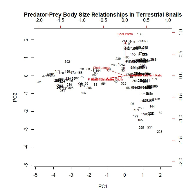 The first principle component separates the data points into two loose groupings, possibly corresponding to our two snail taxa. This component is controlled by shell thickness and predator size, which appear to load strongly together, and by largest fragment ratio, which is negatively correlated with the other two. All three fall almost orthogonal to our second principle component, which is controlled largely by shell width. PC1, therefore, may represent a prey species signal. Cerion snails have thicker shells, are therefore preyed on almost exclusively by larger predators, and are therefore destroyed more thoroughly when killed. On the other hand, shell width varies nearly as much within snail species as it does between species. However, these speculations are all quite tentative. To shed more light on the subject, let us consider a PCA plot of the Cerion snails alone. 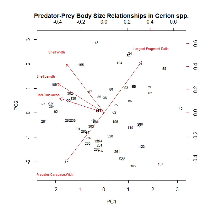 Here a new signal emerges. All of the prey body size variables seem to load together (which makes perfect sense) and, moreover, all three are nearly orthogonal to predator body size. This suggests that, while larger crabs may be more willing to attack a larger, more robust *species* of snail (i.e. Cerion spp.) within that species they show no clear tendency to attack larger, more robust *individuals*. It may be worth nothing that, of the prey body size variables, shell thickness is still most closely aligned with carapace width, but that is a very relative measure. On the other hand, largest fragment ratio is still strongly, negatively correlated with predator body size. The idea that bigger predators are more destructive to shell material seems to hold up well so far. Finally, I plotted a PCA analysis looking only at attacks on H. varians snails. 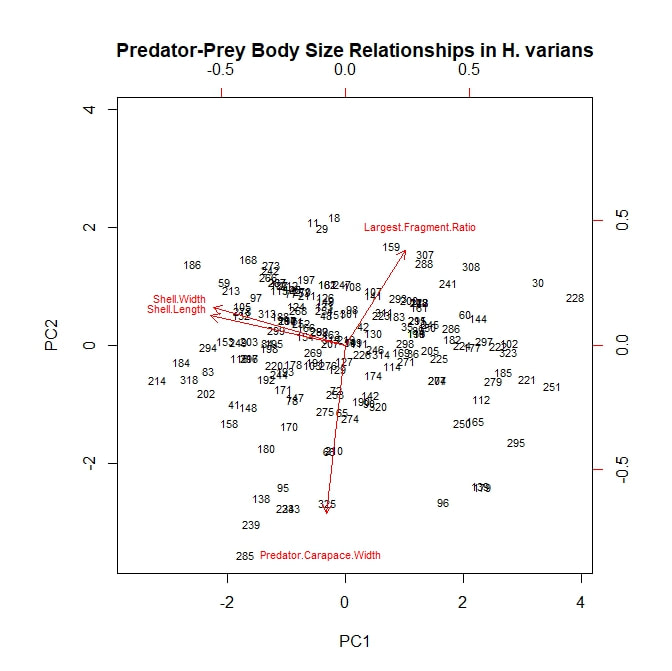 To begin with, it is worth noting that this figure does not consider shell thickness, as any variation within H. varians was beyond the detection limit of the calipers I had on hand. However, the general pattern is similar to that seen in the Cerion snails. Body size variables load together and occur orthogonal to carapace width, which is in turn strongly negatively correlated with largest fragment ratio, providing further support for the tentative theories expressed above.
The most basic analysis I performed during the project was to search for correlated variables. I first imported my data into R, moving them from an Excel spreadsheet to a .txt file along the way. While my data set included a wide range of measurements and observations, for this analysis I limited myself to considering five continuous, numerical variables. Of these, three were body size metrics for the prey animals (i.e.the snails): shell length, shell width, and shell thickness at the aperture. One of the remaining variables was a body size metric for the predators, in this case carapace width. The final variable was a measure I call "Largest Surviving Fragment Ratio". When a snail is attacked or killed, its shell is generally broken. This ratio of the shell's original length to the length of the largest broken fragment gives a rough sense of the extent of the damage done in the attack. I next subset the data by prey species. For this study, only two prey taxa were considered: Hemitrochus varians (also known as the sea grape snail) and Cerion spp. The reason that the Cerion snails (a group made famous by the work of Stephen Jay Gould) were only identified to the genus level is that within the study area of San Salvador Island there are five closely related species of Cerion snails, distinguished by relative few morphological characters and all capable of some degree of hybridization. Thus, identifying any individual to a particular species was impractically difficult. The two snail taxa are quite different, H. varians having delicate, nearly spherical shells while Cerion snails enjoy much sturdier, elongate shells, reinforced with rib-like ornamentation. However, before considering them separately, I first looked to see what patterns emerged when I considered all the snails of both species that were attacked over the course of the experiment. I adapted an R script to produce a correlation matrix (including significance values and scatter plots) with built in displays for the frequency distributions of my five variables. That figure is reproduced below. 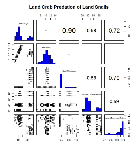 The strongest correlation I observed was between shell length and shell thickness. I interpret this as essentially a species-based signal, as Cerion snails have shells that are both much longer and thicker than those of H. varians. A similar species-based signal can be seen in the bi-modal distributions of many of the variables. In addition, shell length and thickness are correlated with largest fragment ratio. Initially, this seems readily explicable. Thicker (and incidentally longer) shells are sturdier and therefore harder to break into small fragments. However, closer examination shows the correlation observed is actually negative. In other words, sturdier shells are actually being broken into smaller pieces. The exact reason for this signal is difficult to discern, given the species-related overprint, but it may have to do with the secondary correlation between both shell length and width, and predator body size (as represented by carapace width). From this we see that larger, more heavily armored snails are more likely to be the prey of larger crabs. Perhaps it is unsurprising that these more powerful predators, able to tackle sturdy Cerion shells, are also more capable of thoroughly destroying shell material. Moving on, I created a similar figure, looking at the attacks on Cerion snails alone. 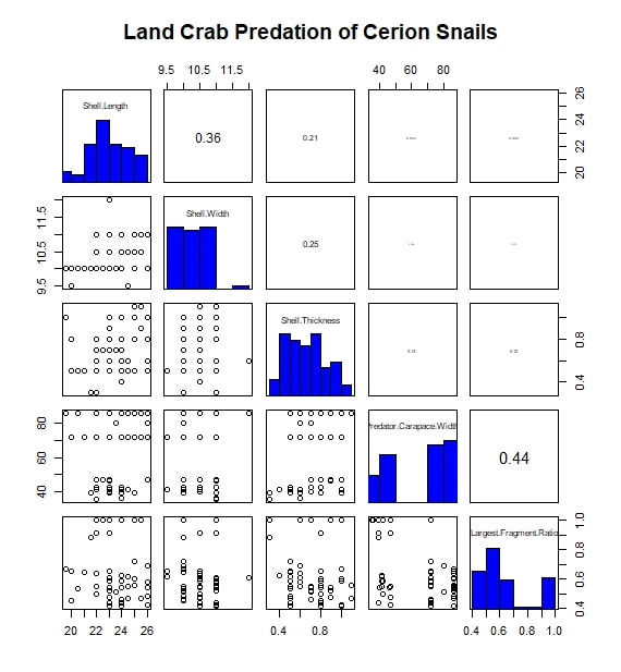 Without a species-related signal, many of the correlations immediately vanish. A weak correlation between shell length and width points to a general body size relationship, while a slightly stronger correlation between predator body size and largest fragment ratio may bear out my earlier theory about the strength and destructive potential of larger crabs. Finally, I considered only the H. varians snails attacked in this experiment. 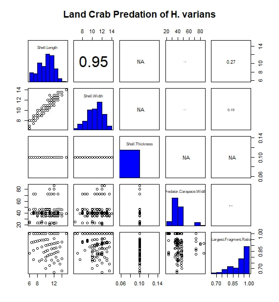 Shell length and width are now strongly correlated, in a testament to H. varians' nearly spherical body plan. Shell thickness does not appear to vary at all; more realistically, any variation was beyond the detection limit of the calipers I had on hand during the experiment. Apart from this, we also see that the largest fragment ratio variable is heavily left-skewed (and is therefore likely the source of the skew observed in the species inclusive version of this figure above). I attempted to address this with several simple transformations. A log transformation proved most effective (yielding the roughly bi-modal distribution seen in the updated correlation matrix seen below) but the skew proved remarkably stubborn. 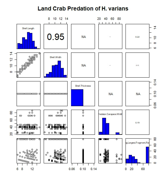 |
JAMES BEECHFirst year Master's student in Geology/Paleontology at WVU. ContentsCategories |
 RSS Feed
